Finding patterns

Week 3 started off with some more improvements to the “skeletonization process”, but soon took a turn towards data analysis. I downloaded some videos from the movement database to the runtime and saved CSV files containing the distances between the head and tail of the worm in form of a time-series.

As seen above, there are two distinct patterns that are observed in the head to tail distances of the “wild” strain and the “unc” strain of the worm. The wild type seems to be more noisy with deeper local minimas. While the changes in the “unc” type are more gradual and predictable.

It is possible to generate a large amount of time series data from the videos that are available on the Movement database. This time series data can be used for 2 possible purposes:

1. First would be to use an LSTM to predict the future sequence of values, a good enough LSTM would be able to find the underlying patterns through the noise.

2. Another possibility would be to use the LSTM to classify the worm’s strain based on the time series data.

I already used a simple LSTM RNN on the time series data as a proof of concept, and here’s how the predictions looked like:

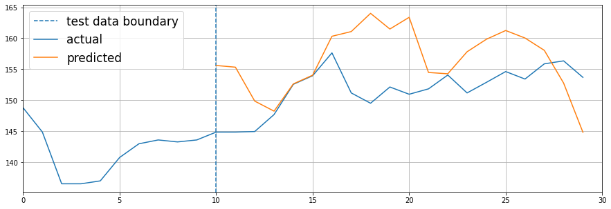
The predictions made aren’t absolutely perfect for now because:

• The dummy model is too small, but it still manages to predict the first quarter of test zone.

• The amount of data used to train the model is relatively low for faster prototyping.

Trying to achieve at least one of these goals would be the goal of the next week.