PCA and semantic segmentation
Week 2 has been the most satisfying week in GSoC yet, with a lot of things getting done. Let’s have a look at them one at a time:
Starting out with semantic segmentation
This is one of the primary objectives of my GSoC project, and it’s about time that I started working on it.
The primary data source would be the WormImage Database, and the objective is to train a model which can segment out the nuclei from the image of an embryo of the C. elegans worm.
The problem is that there’s no labelled segmentation data, only raw images. But I’ve been trying to figure out a way through it, which involves:
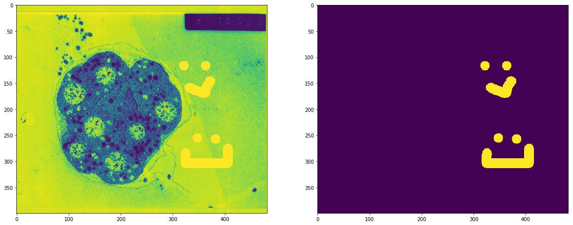
- Taking an original image and manually drawing over the desired parts which are to be extracted. I had to come up with a simple drawing tool which could be used to generate the training masks.
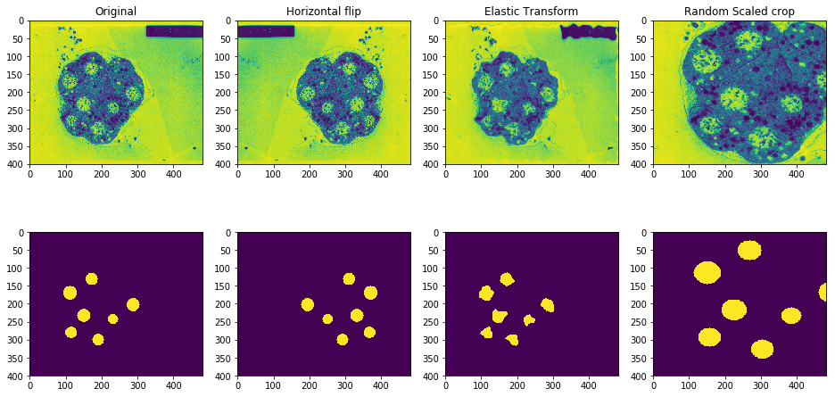
- Run both the original image and the mask through a heavy (but practical) image augmentation pipeline (generate at least 50 images from one)
- Repeat steps 1 and 2 for a few images to get a larger dataset to train on.
I already did steps 1 and 2 on one such image of an embryo and generated a few augmented samples as seen above.
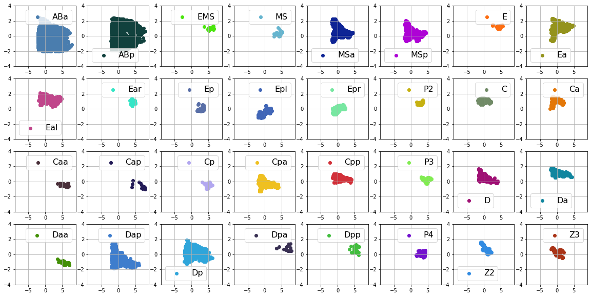
Principal component analysis on embryo metadata
This is where I used some tools like:
-
StandardScaler().fit_transform(x)standardizes the features by removing the mean and scaling them to unit variance. In simpler words, it will transform the data such that its distribution will have a mean value 0 and standard deviation of 1. -
sklearn.decomposition.PCA(n_components = 2)helped in decomposing the 4 dimensional data (x,y,sizeandtime) into a 2 dimensional space while conserving as much information as possible.
Even though 100% of the information from the 4D space could not be projected into the 2 principal components, it gave us a good idea on how cells with similar (or same) lineage ancestors lied closer to each other in the 2D space composed of the 2 principal components.