Training a GAN | Awesome Hugo blog

Training a GAN is an act of balance where we have to balance the generator and the discriminator in a game of losses and probabilities.

The generator:

The generator, when properly trained, takes in random noise as input and returns a sample which would look very similar to the ones from the training distribution. What we’re doing here is basically mapping points a high dimensional distribution to the training samples.

While training, the generator’s main objective is to try to fool the discriminator by generating real looking images.

The discriminator:

The discriminator, when properly trained, would be able to take in an image as an input and return a probability as to whether the image is real or generated. This is more of a classification problem.

While training, the discriminator’s main objective is to distinguish between real and fake images.

Initially when the training starts, both the models are equally bad at their jobs, but in the end pf training, the ideal scenario would be when the generator generators images in-distinguishable from the training set. While the discriminator takes in thatgenerated image and returns a probability of 0.5.

The game of minimax

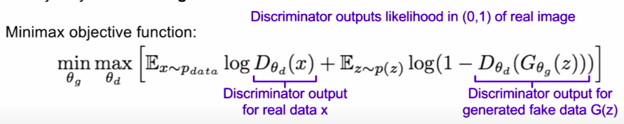
Let’s break down the equation above part by part:

x is the real data
z is the latent vector i.e random noise. It can also be seen as a point in the latent space with n dimensions. For example, torch.randn(64, 1, 1) is a point in the 64 dimensional space.
D(x) is the probability of the original image being real according to the discriminator.
G(z) is the generated image with noise z as input.
D(G(z)) is the probability of the generated image being real according to the discriminator.
E represents the expected value function, the expected value is also known as the expectation, mathematical expectation, mean, average, or first moment.

So what’s going on during training ?

The discriminator wants to maximize D(x) and minimize D(G(z))

The generator wants to maximize D(G(z)) so that the discriminator gets fooled into believing that the generated image is real.

The key factor to maintaining a balance between the 2 model’s capabilities is to choose the right loss landscape.

The training loop:

1. Update discriminator : maximize `log(D(x)) + log(1 - D(G(z)))`

1.1 Backprop the discriminator after feeding real images with labels as 1 (sometimes people also use noisy labels with 1 ± noise) (trying to make D(x) tend towards 1)

1.2 Generate fake images (G(z)) with the generator with random noise z as input.

1.2 Backprop the discriminator after feeding fake images with labels as 0 (sometimes people also use noisy labels with 0 ± noise)

Note: the real and the fake batches were not mixed, first we fed the real batch, and then the fake batch.

2. Update generator: maximize `log(D(G(z)))`

2.1 Use the discriminator’s output on the fake images to calculate a loss with respect to 1. Since the generator’s job is to try to make the discriminator return a 1 on fake images, the closer criterion(discriminator_output, one) is to zero, the better the situation is for the generator.

If you’re more into code than human sentences, here’s a snippet

label.fill_(real_label) # perform another forward pass of all-fake batch through D
output = netD(fake_images).view(-1)
# Calculate G's loss based on this output
errG = criterion(output, label)
# Calculate gradients for G
errG.backward()
D_G_z2 = output.mean().item()
# Update G
optimizerG.step()

If you made it this far, here’s a gif of another model trying to make predictions on the generated images: